Force Analysis of Planar mechanisms

1.1 Force Analysis of Planar mechanisms

1.2 Basic definition

In this chapter we will discuss the methods to do a force analysis (static and dynamic) of a planar mechanism. It is assumed that the students are well aware of the basic concepts of force, moments and vector algebra.

Let us first see the reaction forces and torque that come due to various type of joints. Two links connected by a kinematic joint apply reaction forces (and/or torques) on one another.

1.3 Pin joint

In case of a pin join the reaction forces are equal in magnitude and opposite in direction. The magnitude and direction are determined through proper analysis. Each reaction forces can be further represented in terms of its X and Y component.

1.4 Sliding joint

In the case of a sliding joint the reaction forces are equal in magnitude, opposite in direction, and act perpendicular to the axis of the joint.

1.5 Pin-sliding joint

In case of pin-sliding join the reaction forces are equal in magnitude, opposite in direction, and acts perpendicular to the axis of the joint.

1.6 Static Force Analysis

Here we will deal with scenario where the mechanism is either stationary or operating with a constant velocity, no linear or angular acceleration is associated with the mechanism. This is a case of static equilibrium for the mechanism or the mechanism is in static equilibrium.

1.7 Static equilibrium equations

Planar static equilibrium equations for a single body that is acted upon by forces and torques are expressed as

ΣFi=0=>ΣFi(x)=0andΣFi(y)=0 - - -  (Force equation ) 

ΣTj+ΣMi=0 - - - - - - - - - - - - - - - - - - - - - - - -( Moment equation ) 

Equation (1) represents the sum of all the forces acting on the link, and Equation (2) represents the sum of all the torques and the moments caused by all the forces acting on the body with respect to any reference point.

1.8 Special Cases

When only two or three forces act on a body and the body is in static equilibrium, the forces are balanced in such a way that they exhibit certain characteristics. These are case where it is easier to find the magnitude and direction of the forces and hence we should take advantage of such cases when solving for unknown forces.

Two-force member

If only two forces act on a body that is in staticequilibrium, the two forces are along the axis of the link, equal in magnitude, and opposite in direction.

Three-force member

If only three forces act on a body that is in staticequilibrium, their axes intersect at a single point. A special case of the three-force member is when three forces meet at a pin joint that is connected betweenthree links. When the system is in static equilibrium, the sum of the three forces must be equal to zero.

1.9 Static equilibrium analysis of planar mechanism

We have studied one degree of freedom planar mechanism. These mechanisms can have N number of links and for each link there will be 3 equilibrium equations, which means 3N equation. Our main objective will be to find the unknown reactions/torques with support from the known. We will use the method of free body diagram to develop the 3N equations and then simultaneously solve it. However, sometimes it may be very cumbersome to solve the equations if the numbers of links are many. We will understand the method by taking some example cases.

Case 1: Slider crank mechanism

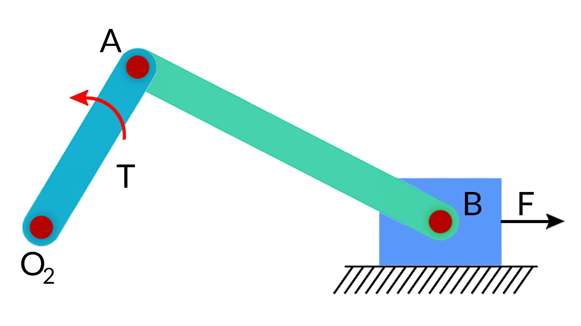
This slider-crank mechanism is in static equilibrium in the shown configuration. A known force F acts on the slider block in the direction shown. An unknown torque acts on the crank. Our objective is to determine the magnitude and the direction of this torque in order to keep the system in static equilibrium.

We construct the free body diagrams for each link.

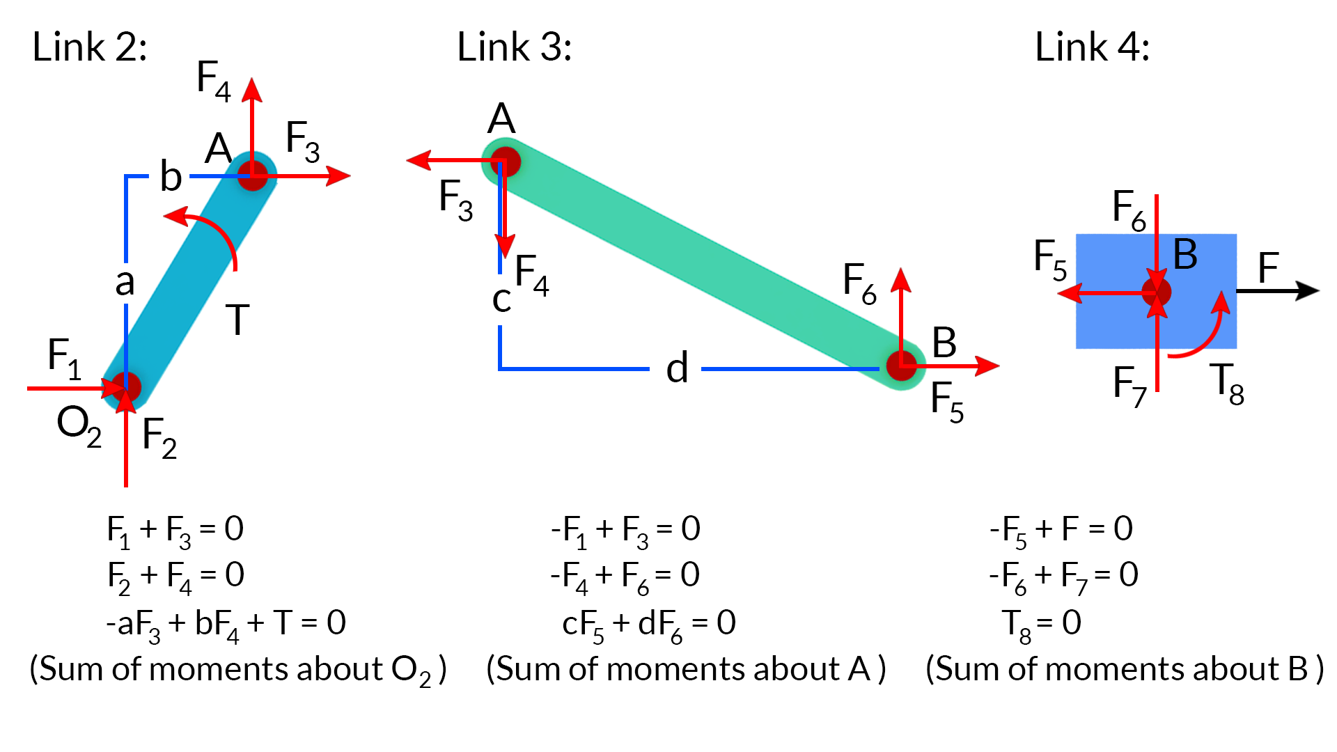
The reaction forces at the pin joints are unknown. Each reaction force is described in term of its x and y components, where the direction of each component is assigned arbitrarily. For notational simplification, simple numbered indices are used for all the components. For each link we construct three equilibrium equations. The moment arms are measured directly from the figure. Note that F7 and T8 are the reaction force and torque due to the sliding joint. These 9 equations can be put into matrix form.

(10100000010100000001010000000ab000010010100000000cd000000010000000001100000000010)(F1F2F3F4F5F6F7T8T)=(000000F00)

The unknowns and their coefficients are kept on the left-hand side and the only known quantity, the known applied force F is moved to the right-hand side. This set of 9 equations in 9 unknowns can be solved by any preferred numerical method. If the arbitrarily assigned direction to a force component or a torque is not correct, the obtained solution will be a negative quantity.

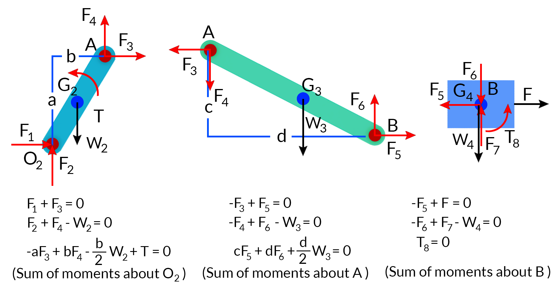
Case 2: Now in the same question of case 1 let us add the effect of gravity and solve again for the unknowns.

The new free body diagram of the links will be as below

These 9 equations are expressed in matrix form and solved for the 9 unknowns by putting them in the matrix form.

(10100000001010000000ab000010010000000001010000000cd000000010000000001100000000010)(F1F2F3F4F5F6F7T8T)=(0W2bW2/20W3dW3/2FW40)

Case 3:

Let us again solve the case 2 by adding frictional force between the slider and ground. 

We see that the FBD of the crank and con rod remains same but the FBD of the slider will change as below

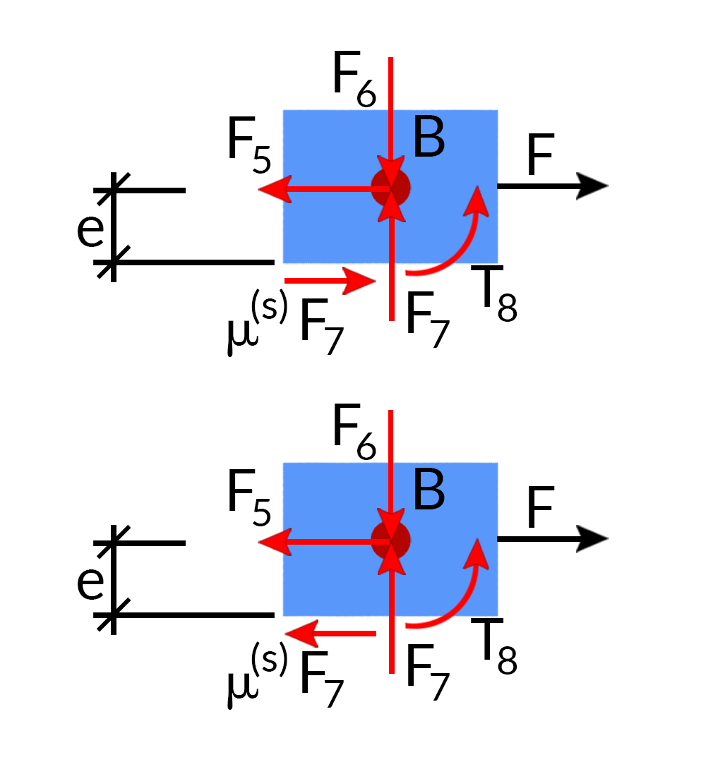
Since frictional force is in the direction against the direction of motion and we are solving for static equilibrium, we will have to take both the cases i.e, when the slider has a tendency to move left and when the slider has a tendency to move right. Corresponding equilibrium equation will also change accordingly

ÀF5+F+Ö(s)F7=0 

ÀF6+F7=0 (The block tends to move to the left) 

T8+eÖ(s)F7=0

ÀF5+FÀÖ(s)F7=0 

ÀF6+F7=0 (The block tends to move to the left) 

T8ÀeÖ(s)F7=0 

The new matrix of 9 equations will be as below

(10100000001010000000ab000010010100000001010000000cd000000010±μ(s)00000001100000000±eμ(s)00)(F1F2F3F4F5F6F7T8T)=(000000F00)

We construct two complete sets of equations for these two cases. The two sets are presented together as shown. We solve each set of equations twice: once with the positive sign in front of μ(s) and once with the negative sign. Each solution yields a value for the unknown torque, Tleft and Tright . As long as the applied torque stays in the range of Tleft to Tright , the system remains in static equilibrium.

1.10 Quick return motion mechanism

In this example, a known force acts at point P an unknown torque acts on the crank. It is assumed that dry friction exists at the sliding joint. To solve this problem, we construct FBD’s for the links. Although it is not necessary, in order to simplify the process of projecting the reaction forces unto the x-y axes, the x-y axes are rotated in such a way that the x-axis is along the axis of link (4).

These equations can be expressed in matrix form and solved twice to find the range of values for the applied torque T.

(10100000001010000000ab000010010±μ(s)00000001010000000001000000±μ(s)01000000100100000c1000)(F1F2F3F4F5F6F7F8T)=(000000Fp(x)Fp(y)dFp)


1.11 Dynamic Force Analysis

As against the static force analysis where the system is set to be in a static state (rest or motion) in dynamic force analysis we will analyse a system which is having some change in its state (again in rest or in motion). In simpler terms the system will have some linear or angular acceleration.

1.12 Dynamic equilibrium equations

Force balancing equation states that when the system is in dynamic state the sum of all forces acting on the body should be equal to the mass of the body, m, times the acceleration of the mass centre, AG.

XFi=mAG=>(PFi(x)=mAG(x) PFi(y)=mAG(y)   

Moment balancing equation states that when a system is in dynamic state the sum of all the moments acting on the body with respect toits mass centre must be equal to the body’s moment of inertia, IG , times the angular accelerationof the body, α. The moment of inertia is defined with respect to an axis passing through themass centre and perpendicular to the plane.

XTj+XMi(G)=IGË 

1.13 D’Alembert’s Principle

Mathematically the D’Alembert principles is just bringing the right hand terms in the dynamic equilibrium equations to the left hand side and equate everything to zero. However, it has profound implications as it means that the sum of all the forces/moments including the inertial force/moment acting on a body in dynamic equilibrium is equal to zero. Which may also mean that there is no difference between the dynamic equilibrium equation and the static equilibrium equations? The revised form of dynamic equilibrium equation as per the D’Alembert’s principle is as below

XFiÀmAG=0 

XTj+XMi(G)ÀIGË=0 

1.14 Dynamic equilibrium analysis of Planar mechanism

The process of conducting a dynamic equilibrium analysis is almost same as the process of static equilibrium analysis except that we need to add the effect of inertial force and inertial torque as shown in the D’Alembert’s principle.

Let us try and understand it better by taking some examples

Case 1: slider crank mechanism

The mass and moment of inertia for the links of this slider-crank are given. A known force F acts on the slider block, and an unknown torque T acts onthe crank. In the depicted configuration, the angular velocity and acceleration of the crank are given. Theobjective is to find the magnitude and the direction of the unknown torque

Based on the given angular velocity and acceleration of the crank, polygons are constructed and the angular velocity and acceleration of all the links are found (magnitudes and directions— ω2 , α2 and α3 are CCW, and ω3 is CW).

Then, in a process similar to that of the static equilibrium the FBD for each link is constructed.

These equations are then put in a matrix form as below

(101000000010100000abab0000100101000000010100000cdcd000000010000000001100000000010)(F1F2F3F4F5F6F7T8T)=(m2AG2(x)m2AG2(y)IG2α(2)m3AG3(x)m3AG3(y)IG3α(3)m4AG4F00)

Case 2: Slider crank mechanism with coloumb force

When frictional force exists between the piston and ground we need to take the effect of frictional force also. The friction force must act in the opposite direction of the motion. The process is illustrated through a simple example.

Since the FBD for the crank and the connecting rod are the same, we only show the FBD for the slider block.

Since, according to the velocity polygon the block ismoving to the left, the friction force must be directed to theright. The equilibrium equations for the block are:

ÀF5+F+Ö(k)F7=m4AG4 

ÀF6+F7=0 

T8+eÖ(k)F7=0

The complete set of equationscan now be presented in matrix form. The solution tothis set of equations yields all the unknowns.

(101000000010100000abab0000100101000000010100000cdcd000000010μ(k)00000001100000000eμ(k)10)(F1F2F3F4F5F6F7T8T)=(m2AG2(x)m2AG2(y)IG2α(2)m3AG3(x)m3AG3(y)IG3α(3)m4AG4F00)


Font Size